Holmes.CaseStudy

Reading: Holmes, T. & Casotto, M, “Penalized Regression and Lasso Credibility,” CAS Monograph #13, November 2024. Chapter 7.

Synopsis: In this article we follow Holmes and Casotto as they embark on a pricing exercise for a fictitious insurer. They construct a synthetic data set with known properties and explore using a GLM and lasso penalized regression to produce a countrywide model. This countrywide model becomes the basis for building state level models via lasso credibility. Four types of state are explored: large, medium, and two versions of a small state. For each type of state they examine the result of (attempting) fitting a GLM, applying penalized lasso regression, and using lasso credibility. We see how lasso credibility allows us to identify credible deviations from the complement even on small data sets where building a GLM is challenging.

Study Tips

This is a long reading with a lot of graphs. Take your time to carefully identify the points highlighted in each graph as we feel this is the type of question you're most likely to see.
Revisit this material frequently because you may not see it often in your day-to-day work.

Estimated study time: 8 Hours (not including subsequent review time)

BattleTable

Based on past exams, the main things you need to know (in rough order of importance) are:

How to compare GLM and lasso penalized regression model output using relativity and pure premium plots.
Convey the importance of using an actuarially sound complement of credibility in a lasso credibility procedure.
Be able to identify when illogical rating occurs and how it can be addressed by tuning the penalty parameter.

Questions from the Fall 2019 exam are held out for practice purposes. (They are included in the CAS practice exam.)

reference	part (a)	part (b)	part (c)	part (d)
Currently no prior exam questions

Full BattleQuiz

Excel Files

Forum

You must be logged in or this will not work.

In Plain English!

Holmes and Casotto provide a case study which demonstrates pricing using both a GLM and a lasso credibility model with simulated data. A log-link function is used consistently throughout. The goal is to highlight the differences between the approaches plus show how lasso credibility is a multivariate credibility based procedure.

The case study begins by building a (U.S.) countrywide model from scratch using a large data set. This model may include a State variable which captures some of the cost differential between states but likely doesn't fully reflect the unique regulations and varying behavior of risk characteristics between states.

Holmes and Casotto then explore what happens when state-level variations are considered. There are three main options available to the modeler:

Small States: Adopt the countrywide model as there is insufficient state-specific data to build a stable model.
Medium States: Adopt the countrywide model with post modeling adjustments for state-specific characteristics. There might just be sufficient data to build a standalone model but it would be time consuming to build a completely separate model as the limited data introduces greater volatility.
Large States: There is usually ample data to build a stable model using only that state's experience.

A GLM does not facilitate blending countrywide and state-specific experience. Post-hoc univariate adjustments of a GLM tend to be less than optimal. On the other hand, lasso credibility provides an easy way for the modeler to blend state-specific experience with the countrywide model in a multivariate setting through including the (transformed) countrywide relativities as offsets.

Description of the Data and Analysis

Holmes and Casotto generated a synthetic commercial auto data set with 3,500,000 records. Risk characteristics were assigned in a way which reflect their real-life univariate distributions and no correlation is assumed between risk characteristics. "True" risk relativities are assigned and then used in conjunction with a base rate to generate "true" pure premium. Finally, an "experienced" pure premium is simulated from this via a Tweedie distribution.

Figure 7.1 below shows their 3,500,000 records with the insurer's largest state (green), one of their medium states (yellow), and two small states (red) highlighted. The remaining 2,500,000 records come from a variety of states of which none are as large as the green block. The first highlighted small state is deliberately simulated to have different risk relativities to the base modeling data while the second small state is simulated with the same underlying risk relativities. The goal of these two small states is to show for the first one that lasso credibility can pick up meaningful differences while for the second, lasso credibility creates a sparse model.

By using a synthetic data set where the true relativities are known, there is no need for Holmes and Casotto to partition their data into modeling and validation data sets.

Figure 7.1

To keep the project manageable, Holmes and Casotto use the following limited number of variables: Driver Age, Vehicle Age, Industry Code, Vehicle Weight, Multi-Policy Discount, and x-Treme Turn Signal.

Despite Holmes and Casotto's earlier warnings, Driver Age and Vehicle Age are treated as continuous variables while the remaining variables are categorical. Driver Age and Vehicle Age are modeled using three and two piecewise linear functions respectively.

The following graphs show the true risk relativities selected by Holmes and Casotto for their base data, large state, medium state, and first small state. You can click on each graph to enlarge it.

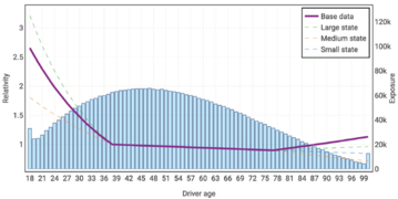
Driver Age
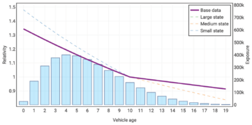
Vehicle Age
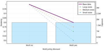
Multi-Policy Discount
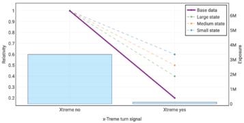
x-Treme Turn Signal
Vehicle Weight
Industry

As you look at the above true relativities you should observe the following:

Driver Age: The data is thin once the age is in the 80s.
Vehicle Age: The data is very thin for the oldest ages.
Multi-Policy Discount: The underlying data is constructed to always have a discount present in every cut of the modeling data.
x-Treme Turn Signal: This is a fictitious feature which was recently introduced to the insurer's book of business. It has a very low relativity (highly predictive) but also incredibly low exposure.
Vehicle Weight: This could have been modeled as an ordinal variable but is categorical. The Extra-Light category will be very hard to model due to the small exposure volume.
Industry: None of these categories lend themselves to being combined with another so it's best to model them all separately. The Firework category has very few exposures but is known to require a high relativity.

Question: Identify five advantages of using a synthetic/simulated data set to compare the GLM and lasso credibility models.

Solution:

The true underlying relativities are known (and shown above). Lift charts can be made to compare the model against the true values rather than potentially noisy validation data.
The risk characteristics are known to be uncorrelated so correlation does not affect either the GLM or lasso credibility models used.
The case study can correctly highlight situations where lasso credibility performs well and where it doesn't. Further, we can understand why this type of performance is exhibited.
The correct variable transformations to capture the true risk characteristics are known. This simplifies the feature engineering process, allowing the focus to remain on the differences between the GLM and lasso credibility approaches.
The underlying data can be resimulated for additional investigation.

Holmes and Casotto use the same feature engineering (selected variables) in both their GLMs and lasso credibility models. Each lasso credibility model has its penalty parameter selected using cross-validation and coefficients are standardized.

Holmes and Casotto ignore traditional ways of measuring GLM performance such as deviance or the Gini coefficient. This is because they know the true relativities so we gain more insight by comparing the indicated and simulated relativities to the true relativities.

When using relativity plots with true relativities, the model which produces relativities closest to the true relativities is the better performing model.

Holmes and Casotto also use prediction plots which show the true pure premium, experienced (simulated) pure premium, GLM pure premium, and lasso credibility predicted pure premium. Double lift charts are also used to compare models — the model which is closest to the horizontal line at 1.0 is the better performing model.

Countrywide Model

Holmes and Casotto build a GLM and a lasso penalized regression model on the full 3,500,000 record data set. Penalized regression is used rather than lasso credibility because there is no known complement available at this point. Figure 7.2 below shows the coefficients resulting from these models on the countrywide data set.

Table 7.2: Countrywide GLM and lasso penalized regression model output

The key thing to notice from Table 7.2 is all of the lasso penalized regression coefficients except for driver_age_18_38_hinge and ind_food_services are slightly closer to zero than the GLM coefficients. Since the GLM result is considered 100% credible, having penalized coefficients close to the GLM result tells us penalized regression is assigning a lot of credibility. This is not too surprising given we have a large data set at this point and in theory the experience is stable.

Alice: "You may notice driver_age_18_38_hinge has identical GLM and penalized regression results. This is saying that variable is 100% credible (up to rounding at least). The odd one out is ind_food_services which has a penalized regression coefficient that is further away from zero than the GLM coefficient is. This seems to be a typo — we're confirming this with Holmes and Casotto."

The source tells us (but doesn't show) the p-values for the countrywide model are all smaller than 0.05, i.e. all variables are highly significant.

Figures 7.8 and 7.9 below show the relativity and pure premium plots respectively for the Industry variable. The penalized lasso regression points are virtually indistinguishable from the GLM points (as discussed above). What stands out is there are material deviations from the true result (purple) for the Fireworks and Health Care industries. Both models have materially overpredicted those relativities. The pure premium plot tells us why — the simulation process produced experienced pure premiums which are significantly higher than the true pure premiums and both the GLM and penalized lasso regression models have reacted to this signal in the observed data. The models reacted to the signal despite it really being a matter of unlucky experience.

Figure 7.8: Industry relativity plot for countrywide models

Figure 7.9: Industry pure premium plot for countrywide models

Figure 7.10 below shows the quantile plot for the countrywide GLM and penalized lasso regression models. Performance is very close and it takes a double lift chart (Figure 7.11 below) to really tell which performs best (the GLM does by a tiny margin).

Figure 7.10: Quantile plot for countrywide models

Figure 7.1: Double lift chart for GLM and lasso penalized regression countrywide models

Alice: "A technical detail — we've been calling it lasso penalized regression so far instead of lasso credibility. Yet we saw earlier that lasso credibility can choose to use zero as the complement of credibility. So why not call it lasso credibility? According to Holmes and Casotto we shouldn't call it lasso credibility because we have no actuarial justification (yet) for choosing zero to be the complement of credibility. We should only call it lasso credibility when we can justify the choice of complement."

Modeling the Large State

Having determined an appropriate countrywide model (Holmes and Casotto don't say which of the GLM and lasso penalized regression models they ultimately chose), we turn our attention to modeling the rating plan for the insurer's largest state.

We have three options, build a:

Standard GLM model,
Lasso penalized regression model,
Lasso credibility model where the complement of credibility comes from the relativities found in our countrywide model.

We assume that, although this is the insurer's largest state, it does not have an outsized influence on the countrywide model.

First, we compare the standard GLM model with the lasso penalized regression on model on the large state data set. We're told the p-values for driver_age_76_99_hinge and vehicle_age_10_99_hinge are now greater than 0.05, indicating the countrywide GLM model isn't stable any more. Figure 7.12 below shows how the tail of the driver age variable isn't picking up the true signal very well. The GLM does a better job because the lack of credibility in the tail means the lasso penalized regression coefficient is brought closer to 0 which flattens the slope. However, it remains that the GLM coefficient for the tail is not significant, so the modeler should refit using a different transformation of the Driver Age variable.

Figure 7.12

We see a similar situation in the tail of the Vehicle Age variable where neither the GLM or the lasso penalized regression pick up much of the true signal after vehicle age 10 (see Figure 7.13 below).

Figure 7.13

In both of Figures 7.12 and 7.13 we see the slope of the lasso penalized regression model in the tail is flatter than the slope of the GLM model in the tail. This is the correct behavior as recall Holmes and Casotto made the decision to include these variables as continuous variables in the model.

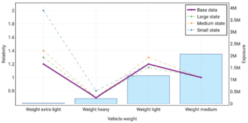
In Figure 7.14 below we see the extra light vehicle weight relativity has been shrunk towards 1.000 in the lasso penalized regression model. This reflects the associated low exposure volume. We're told the p-value for the extra light vehicle weight category is just below 0.05.

Figure 7.14

In each of Figures 7.12, 7.13, and 7.14 we've seen the lasso penalized regression model captures some of the signal. The amount of shrinkage (towards the zero coefficient/relativity of e⁰ = 1.000) increases as the exposure volume decreases.

Since some of the GLM coefficients now have p-values greater than 0.05 we're faced with two options. Either keep the insignificant variables in our GLM so the structure is the same as the countrywide model, or remove the insignificant variables and refit the GLM.

Due to the way Holmes and Casotto approach this case study, we know the true relativities so can assess which of these approaches is better in this case. Figure 7.15 below shows the GLM which includes the insignificant variables performs better than the lasso penalized regression model. However, Figure 7.16 below shows that once we remove the insignificant variables and refit the GLM, the lasso penalized regression model outperforms this new GLM.

Alice: "The key point Holmes and Casotto are making here is it's better to have some credibility (lasso penalized model) than it is to have none assigned (updated GLM)."

Figure 7.15: The GLM includes the insignificant variables

Figure 7.16: The GLM has been refitted without the insignificant variables

Now let's look at the lasso credibility model where we used the countrywide relativities to produce the complement of credibility. By using the countrywide complement we are really modeling credible differences between the large state and the countrywide model rather than building an entirely new model from scratch. The extra information produces a more robust model.

The table below shows a comparison of the various model relativities for the Industry rating variable

Description	Farming	Food Service	Construction
Exposures	75,000	380,000	200,000
Complement of Credibility	0.680	1.205	1.460
Lasso Credibility	0.680	1.205	1.436
True Relativity	0.700	1.200	1.400
GLM Relativity	0.668	1.171	1.379

In the above table we see the lasso credibility relativities are identical to the complement of credibility for the Farming and Food Service categories (no credible difference from the complement). This indicates the [math]\beta_j[/math] coefficients are zero in the model so these categories received either zero credibility or the model had very high confidence in the complement of credibility. In contrast, the Construction category there is a material difference between the GLM, lasso credibility, and complement of credibility relativities. Although the exposure volume is relatively small, the variation in the beta coefficient for this category outweighs the increase in the penalty term and we move away from the GLM relativity towards the complement of credibility, bringing us closer to the true relativity, avoiding the overreaction present in the GLM. In this context, lasso credibility provides stability which may prevent unnecessarily large policyholder impacts arising from assigning too much credibility to noisy data.

As expected, we also see the lasso credibility model producing results for categories with high levels of exposure that are closer to the GLM relativities than the complement. Figure 7.18 below shows this for the Multi-Policy Discount variable.

Figure 7.18

The key takeaway to remember is not all components of the complement of credibility will be equally influential on the model results. Further, while credibility procedures are often effective, it's still possible for noisy data to cause the indicated relativities to be further away from the true relativities than we'd like.

We now use double lift charts to compare the lasso credibility model to the GLM and the lasso penalized regression models. The GLM model includes insignificant variables (those with p-values greater than 0.05).

Figure 7.21: Performance against the GLM

Figure 7.22: Performance against the lasso penalized regression model

Lasso credibility is not guaranteed to outperform other types of model. It is highly dependent on an appropriate choice of complement when the data is thin. This is best seen in the following comparison table

Description	Farming	Health Care
Exposures	75,000	25,000
True Relativity	0.700	1.200
GLM Relativity	0.668	1.165
Complement of Credibility	0.680	1.399
Lasso Credibility	0.680	1.288
Lasso Penalized Regression	0.718	1.101

The key takeaways from the above table are:

Farming has more exposures than Health Care so choosing a poor complement relativity (0.680 or 1.000) had less of an impact as the results are within 0.02 of the true relativity.
The GLM relativity is better for Health Care (closer to the true relativity) because we made a poor choice for the complement (1.399 or 1.000) —in each case the complement is quite far away from the true relativity and the signal in the data was insufficient to overcome our choice of complement.

Alice: "You didn't forget lasso penalized regression means the complement coefficient is 0 which, with a log link function, means the complement relativity is 1.000 — did you?"

Question: Identify when lasso credibility should outperform a GLM.

Solution: Lasso credibility should outperform a GLM when the complement of credibility pulls the indicated relativities in the correct direction, i.e. towards the true relativities.

Question: Identify when lasso credibility should outperform lasso penalized regression.

Solution: Lasso credibility should outperform lasso penalized regression when the complement of credibility is more appropriate than the default assumption of 1.000.

Alice: "A poor choice of complement can cause lasso credibility to perform worse than a GLM or lasso penalization regression."

We've seen that even on a large subset of our initial modeling data that fitting the same GLM results in smaller categories now receiving insignificant coefficients. We've also seen how lasso credibility with an appropriate complement of credibility allows us to produce a better model even though we have a lot of data. Let's now look at what happens with less data in a medium size state which is growing.

Modeling the Medium State

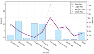
With a smaller data set, fitting the countrywide GLM model results in more coefficients having non-significant p-values. Further, some of the results become directionally incorrect. We see this for the Industry rating variable in Figure 7.23 below.

Figure 7.23: Industry relativities for the medium state GLM

In Figure 7.23 above we see the Fireworks and Real Estate categories have GLM indicated relativities which are directionally opposite to both the complement and true relativities (discount for Fireworks when it should be a surcharge, and a surcharge for Real Estate when a discount is merited). Even the lasso credibility model gets the direction wrong for Fireworks and produces a Real Estate relativity which is a material distance from both the true result and the complement. According to Holmes and Casotto, this means we need to adjust the penalty parameter to correct for the illogical Fireworks result.

Alice: "In real life we don't know the true relativities so the focus here is on looking at where the complement relativities are directionally opposite to the GLM and/or lasso credibility relativities."

Since Figure 7.23 shows the Fireworks lasso credibility relativity being much closer to the GLM result than the complement, this tells us we need to reduce the assigned credibility. In other words, we must increase the lambda parameter to give more credibility to the chosen complement by making it harder for the beta coefficient to move away from zero and hence away from the complement. This emphasizes why it's important to carefully review the relativity plots when finalizing the lambda parameter.

Alice: "Holmes and Casotto note that the GLM result for Fireworks is a relativity of 0.01 with a p-value of 0.0645. Critically, this is really close to our arbitrary p-value threshold of 0.05. If the modeler wasn't looking for illogical rating they could accidentally use the GLM to give a discount to Fireworks!"

Increasing the penalty parameter greatly improves the lasso credibility output as we see in Figure 7.26 below.

Figure 7.26: Industry relativities for the medium state GLM after tuning the lambda parameter

This illustrates a key benefit of lasso credibility. It allows us to find credible differences in a state's experience from a countrywide model. We also avoid the temptation to implement the countrywide model as is rather than sinking considerable time and energy into coming up with feature engineering that would allow us to produce a reasonable GLM for the medium state.

Lasso credibility doesn't cure everything though. In tail of Figure 7.24 and in Figure 7.25 (shown below) we see the GLM would still have performed better and the lasso credibility has recognized some but not enough of the signal present. Unfortunately for the GLM, the p-values associated with these results are insignificant so we'd likely have rejected the coefficients in favor of a different model.

Figure 7.24

Figure 7.25

Lasso credibility allows us to build better models on smaller data sets because it incorporates prior assumptions and assigns partial credibility to coefficients rather than assigning full credibility to all significant coefficients.

Modeling the Small States

The countrywide GLM model has 19 coefficients in it and attempting to fit this model to one of the small state data sets results in nine of these coefficients being insignificant. We'd quickly give up building a GLM! We initially focus on the first small state which we know has different true relativities to the base countrywide model. Again, rather than adopting the countrywide GLM, we can use lasso credibility to build state specific models which perform better (see Figure 7.29 below)

Figure 7.29

Fine tuning the penalty parameter by increasing it can help prevent overreaction to the noise present in the small data set. This is seen in Figure 7.30 below in which the lasso credibility line is closer to the true line than it was when using a smaller penalty parameter in Figure 7.29 above.

Figure 7.30

Now returning to the second small state which we know has approximately the same true relativities to the base countrywide model. The lasso credibility output is entirely zeroes! Every single variable has been penalized out to produce the underlying countrywide model that was used as the offset.

We can only tell that there should be no credible difference between the second small state and the countrywide model through the use of lasso credibility and looking for credible deviations from the countrywide model. We couldn't even consider using significance because building a suitable GLM on such thin data is practically impossible.

Holmes and Casotto conclude with small data sets we aren't "fully justifying new rates" when we use lasso credibility. Instead, we are "identifying credible differences for further investigation".

Question: Briefly describe two key advantages of being able to apply lasso credibility to small data sets.